
The SVG 2.0 Draft include a new graphical element/texture: the Gradient Mesh. While not a novel technique, postscript use them as ShadingType 6 and 7 (Coons patch meshes and Tensor product patch meshes) as well as PDF PDF (section 4.6.3), it's implementation details and understanding are worthwhile.
This document will describe how is defined a Gradient mesh within the SVG 2 draft specification, describes how to render it, look at the Postscript/PDF extension for tensor product and, finally the other possible extension for the tool.
Keep your pomax guide to the bezier curve nearby and Let's roll.
If you didn't click the links in the introduction, you might still be wondering what is the gradient mesh, to explain it, let's take an axis aligned grid, composed of vertices and edges:
Now let's loosen the definition by swapping axis aligned line with (cubic) bezier curves. We also choose to be free in the position of the vertices:

While funky lines are relatively interesting in their own rights, they are not that interesting for a shading, so we associate a color to the vertices of the grid:

For every cell of the array, we want to fill it by interpolating the colors of the vertices, by following the curves, possibly producing curved gradients along the way:

So here we are with our first gradient mesh. Defined by 5 by 4 vertices and their associated colors and the bezier control points for the edges. A cell of this array define a Coon patch, so 4 vertices and 4 edges and 4 colors. Knowing how to render one coon patch gives the key to render the whole mesh, you just render each cell individually.
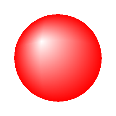
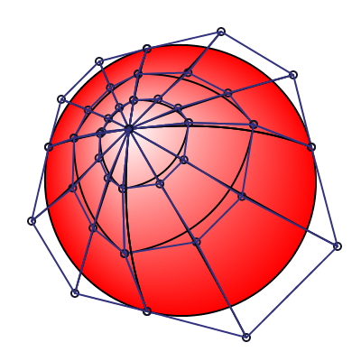
We are now focusing on a single coon patch:
The black circle are the vertice from the mesh patch, and the dark blue one not in the corner are the control points for the cubic bezier curves, The control mesh is drawn in dark blue.

We can see that the color are the strongest in the corners, which correspond to the vertice of the mesh.
The main idea is then to subdivide this patch up to a point where either it is too small for further subdivision (if we are below the size of pixel for instance) or if further subdivision won't refine color, if color are too close we are not really interested.

Managing to subdivide a coon patch in quadrant, means we can render our coon patch. To represent coon patch in Haskell, we'll use the following data types:
--
-- @
--                        ----->
--                  North     _____----------------+
--   ^          +------------/                     /
--   |         /                                  /       |
--   |        /                                  /        |
--   |       /                                  /  east   |
--   | west |                                  /          |
--          |                                 |           v
--           \                                 \   .
--            \                  __-------------+
--             +----------------/
--                    South
--                       <-----
-- @
--
data CoonPatch colors = CoonPatch
    { _north :: !CubicBezier
    , _east :: !CubicBezier
    , _south :: !CubicBezier
    , _west :: !CubicBezier
    , _coonValues :: !colors
    }
    deriving Show
CoonPatch represent the geomentry along with the colors stored in _coonValues. We can argue that this storage is redundant because the first and last point of each cubic bezier are shared, but manipulating a CubicBezier data types make things easier down the line. To store the colors we use another data type:
-- | Values associated to the corner of a patch
-- @
--  North           East
--      +----------+
--      |0        1|
--      |          |
--      |          |
--      |3        2|
--      +----------+
--  West            South
-- @
data ParametricValues a = ParametricValues
  { _northValue :: !a
  , _eastValue  :: !a
  , _southValue :: !a
  , _westValue  :: !a
  }
  deriving (Functor, Show)
A fully instantiated type for a coon patch may then be CoonPatch (ParametricValues PixelRGBA8) (Using the pixel type from JuicyPixels)
A CubicBezier in encoded the following way:
type Point = V2 Float

-- | Describe a cubic bezier spline, described
-- using 4 points.
--
-- > stroke 4 JoinRound (CapRound, CapRound) $
-- >    CubicBezier (V2 0 10) (V2 205 250) (V2 (-10) 250) (V2 160 35)
--
-- <<docimages/cubic_bezier.png>>
--
data CubicBezier = CubicBezier
  { -- | Origin point, the spline will pass through it.
    _cBezierX0 :: !Point
    -- | First control point of the cubic bezier curve.
  , _cBezierX1 :: !Point
    -- | Second control point of the cubic bezier curve.
  , _cBezierX2 :: !Point
    -- | End point of the cubic bezier curve
  , _cBezierX3 :: !Point
  }
  deriving Eq
V2 being the Linear type for two component vector.
We can now look to the mathematical definition of the coon surface, which is defined by a simple equation:
\[ S = S_C + S_D - S_B \]
with each subsurface like:
                    C                            C (1)
        C (0)        1    _____----------------+  1
         1  +------------/                     /
           /                                  /
          /                                  /
         /                                  /  D
   D    |                                  /    2
    1   |                                 |
         \                                 \
          \                  __-------------+
           +----------------/                C (1)
      C (0)             C                     2
       2                 2
\[ S_C(u, v) = (1 - v) × C_1(u) + v × C_2(u), \\ S_D(u, v) = (1 - u) × D_1(v) + u × D_2(v), \\ S_B(u, v) = (1 - v) × [(1 - u) × C_1(0) + u × C_1(1) ] + v * [(1 - u) × C_2(0) + u × C_2(1)] \]
We can see that \(S_C\) is a linear interpolation between the top and bottom bezier curve, \(S_D\) a linear interpolation between the left and right curve.
Finally, \(S_B\) is a bilinear interpolation between the four corner of the coon patch. So by introducting a lerp function, we can rewrite the surfaces:
\[ S_C(u, v) = lerp(v, C_1(u), C_2(u)), \\ S_D(u, v) = lerp(u, D_1(v), D_2(v)), \\ S_B(u, v) = lerp(v, lerp(u, C_1(0), C_1(1)), lerp(u, C_2(0), C_2(1))) \]
The \(u\) and \(v\) parameters are moving freely from 0 to 1 and are the UV coordinate inside the patch.
With this definition at end, we can write a function to get back a single point out of the surface:
-- | Return a postion of a point in the coon patch.
coonPointAt :: CoonPatch a -> UV -> Point
coonPointAt CoonPatch { .. } (V2 u v) = sc ^+^ sd ^-^ sb
  where
    CubicBezier c10 _ _ c11 = _north
    CubicBezier c21 _ _ c20 = _south

    sc = lerp v c2 c1
    sd = lerp u d2 d1
    sb = lerp v (lerp u c21 c20)
                (lerp u c11 c10)

    CubicBezier _ _ _ c1 = fst $ cubicBezierBreakAt _north u
    CubicBezier _ _ _ c2 = fst $ cubicBezierBreakAt _south (1 - u)

    CubicBezier _ _ _ d2 = fst $ cubicBezierBreakAt _east v
    CubicBezier _ _ _ d1 = fst $ cubicBezierBreakAt _west (1 - v)
It uses the Linear library, with the ^+^ adding two vectors by performing pairwize addition, ^-^ doing pairwise subtraction. For the renderer, we want to divide the coon patch up to the pixel level, so we will use another algorithm than sampling this function.
A little note on the lerp doing a linear interpolation between two vectors, it's current behaviour is the following one
lerp 0 a b = b
lerp 1 a b = a
So the use of lerp may appear "reversed" compared to others lerp definitions (and from the one in our formulas)
We can use De Casteljau's algorithm to split a cubic bezier curve in two, as our degree is known, we can directly unroll the implementation:
midPoint :: Point -> Point -> Point
midPoint a b = (a ^+^ b) ^* 0.5

divideCubicBezier :: CubicBezier -> (CubicBezier, CubicBezier)
divideCubicBezier bezier@(CubicBezier a _ _ d) = (left, right) where
  left = CubicBezier a ab abbc abbcbccd
  right = CubicBezier abbcbccd bccd cd d
  (ab, _bc, cd, abbc, bccd, abbcbccd) = splitCubicBezier bezier

splitCubicBezier :: CubicBezier -> (Point, Point, Point, Point, Point, Point)
splitCubicBezier (CubicBezier a b c d) = (ab, bc, cd, abbc, bccd, abbcbccd)
  where
    --                     BC
    --         B X----------X---------X C
    --    ^     /      ___/   \___     \     ^
    --   u \   /   __X------X------X_   \   / v
    --      \ /___/ ABBC       BCCD  \___\ /
    --    AB X/                          \X CD
    --      /                              \
    --     /                                \
    --    /                                  \
    -- A X                                    X D
    ab = a `midPoint` b
    bc = b `midPoint` c
    cd = c `midPoint` d

    abbc = ab `midPoint` bc
    bccd = bc `midPoint` cd
    abbcbccd = abbc `midPoint` bccd
We introduce a new Linear operator ^* which multiplies all the component of the vector (on the left) by the scalar on the right. We can also easily represent a straight line using a cubic bezier curve:
straightLine :: Point -> Point -> CubicBezier
straightLine a b = CubicBezier a p1 p2 b where
  p1 = lerp (1/3) b a
  p2 = lerp (2/3) b a
We can also flip the direction of a cubic bezier curve, without altearing it's appearance
inverseBezier :: CubicBezier -> CubicBezier
inverseBezier (CubicBezier a b c d) = CubicBezier d c b aTo split a coon patch in two, we have to know how to produce a new cubic bezier between the two new patch. Splitting a cubic bezier for the edges will use the function defined above. We will use the algorithm described in the paper "An efficient algorithm for subdividing linear Coons surfaces"[1].
The main hindsight gained from the paper is how to calculate the contribution of \(S_D\) when spliting \(S_C\) in two. The linear part (\(S_B\)) is still a bilinear interpolation, the \(S_C\) part is a direct interpolation of \(C_1\) and \(C_2\).
The contribution of \(S_D\) when splitting \(S_C\) is in fact a straight line with endpoints the middle of \(D_1\) and \(D_2\). With these contribution, the regular equation for \(S\) can be applied. It can be noted that the paper use a notation involving cardinal points which have been used when defining the various data types.
The combination is then stated by the definition below:
-- | Calculate the new cubic bezier using equation for S
combine :: CubicBezier -> CubicBezier -> CubicBezier -> CubicBezier
combine (CubicBezier a1 b1 c1 d1)
        (CubicBezier a2 b2 c2 d2)
        (CubicBezier a3 b3 c3 d3) =
  CubicBezier (a1 ^+^ a2 ^-^ a3)
              (b1 ^+^ b2 ^-^ b3)
              (c1 ^+^ c2 ^-^ c3)
              (d1 ^+^ d2 ^-^ d3)
And the proper subdivision for the coon patch is then:
-- | Split a coon patch in two vertically
--
-- @
--                        --------->
--                  North     +____----------------+
--   ^          +------------/:                    /
--   |         /              :                   /       |
--   |        /               :                  /        |
--   |       /               :                  /  east   |
--   | west |               :                  /          |
--          |               :                 |           v
--           \               :                 \    .
--            \               :  __-------------+
--             +--------------+-/
--                    South
--                       <---------
-- @
--
subdividePatch :: CoonPatch (V2 CoonColorWeight)
               -> Subdivided (CoonPatch (V2 CoonColorWeight))
subdividePatch patch = Subdivided
    { _northWest = northWest
    , _northEast = northEast
    , _southWest = southWest
    , _southEast = southEast
    } where
  north@(CubicBezier nw _ _ ne) = _north patch
  south@(CubicBezier se _ _ sw) = _south patch

  -- Midpoints used for S_B
  midNorthLinear = nw `midPoint` ne
  midSouthLinear = sw `midPoint` se
  midWestLinear = nw `midPoint` sw
  midEastLinear = ne `midPoint` se

  -- These points are to calculate S_C and S_D
  (northLeft@(CubicBezier _ _ _ midNorth), northRight) = divideCubicBezier north
  (southRight, southLeft@(CubicBezier midSouth _ _ _ )) = divideCubicBezier south
  (westBottom, westTop@(CubicBezier midWest _ _ _)) = divideCubicBezier $ _west patch
  (eastTop@(CubicBezier _ _ _ midEast), eastBottom) = divideCubicBezier $ _east patch

  -- This points are to calculate S_B
  midNorthSouth = north `midCurve` south
  midEastWest = _east patch `midCurve` _west patch

  -- Here we calculate S_D sub curves
  (splitNorthSouthTop, splitNorthSouthBottom) =
      divideCubicBezier $ combine
        midEastWest                                     -- S_D
        (midNorth `straightLine` midSouth)              -- S_C contribution
        (midNorthLinear `straightLine` midSouthLinear)  -- S_B contribution

  (splitWestEastLeft, splitWestEastRight) =
      divideCubicBezier $ combine
        midNorthSouth                                   -- S_C
        (midWest `straightLine` midEast)                -- S_D contribution
        (midWestLinear `straightLine` midEastLinear)    -- S_B contribution

  weights = subdivideWeights $ _coonValues patch

  -- reconstruction of the new sub-patches.
  northWest = CoonPatch
    { _west = westTop
    , _north = northLeft
    , _east = splitNorthSouthTop
    , _south = inverseBezier splitWestEastLeft
    , _coonValues = _northWest weights
    }

  northEast = CoonPatch
    { _west = inverseBezier splitNorthSouthTop
    , _north = northRight
    , _east = eastTop
    , _south = inverseBezier splitWestEastRight
    , _coonValues = _northEast weights
    }

  southWest = CoonPatch
    { _west = westBottom
    , _north = splitWestEastLeft
    , _east = splitNorthSouthBottom
    , _south = southLeft
    , _coonValues = _southWest weights
    }

  southEast = CoonPatch
    { _west = inverseBezier splitNorthSouthBottom
    , _north = splitWestEastRight
    , _east = eastBottom
    , _south = southRight
    , _coonValues = _southEast weights
}The coon function use a subdivideWeights function to subdivide the weight at the corner of the patch, this is a straightforward operation, the ParametricValues data type is a generic data type storing values for the four corner of the patch. We don't directly interpolate pixels, but instead the UV parametric coordinate within the patch. Subdividing it is just creating new squares with new coordinate using midPoints.
subdivideWeights :: ParametricValues (V2 CoonColorWeight)
                 -> Subdivided (ParametricValues (V2 CoonColorWeight))
subdivideWeights values = Subdivided { .. } where
  ParametricValues
    { _westValue = west
    , _northValue = north
    , _southValue = south
    , _eastValue = east
    } = values

  --  N       midNorth    E
  --      +-------+------+
  --      |0      :     1|
  --   mid|   grid:Mid   |
  --  West+=======:======+ midEast
  --      |       :      |
  --      |3      :     2|
  --      +-------+------+
  --  W       midSouth    S
  midNorthValue = north `midPoint` east
  midWestValue = north `midPoint` west
  midSoutValue = west `midPoint` south
  midEastValue = east `midPoint` south

  gridMidValue = midSoutValue `midPoint` midNorthValue

  _northWest = ParametricValues
    { _northValue = north
    , _eastValue = midNorthValue
    , _southValue = gridMidValue
    , _westValue = midWestValue
    }

  _northEast = ParametricValues
    { _northValue = midNorthValue
    , _eastValue = east
    , _southValue = midEastValue
    , _westValue = gridMidValue
    }

  _southWest = ParametricValues
    { _northValue = midWestValue
    , _eastValue  = gridMidValue
    , _southValue = midSoutValue
    , _westValue = west
    }

  _southEast = ParametricValues
    { _northValue = gridMidValue
    , _eastValue = midEastValue
    , _southValue = south
    , _westValue = midSoutValue
    }
It is assumed that the original weight are a unit square:
 0,0                1,0
    +--------------+
    |              |
    |              |
    |              |
    |              |
    |              |
    +--------------+
0,1 1,1We just need a way to convert between UV coordinates to real color to fill our canvas, it is rather simple, if we store the initial pixel in ParametricValues, we just have to perform a bilinear interpolation to get the final color:
meanValue :: ParametricValues (V2 CoonColorWeight) -> V2 CoonColorWeight
meanValue = (^* 0.25) . getSum . foldMap Sum

-- | Interpolate a 2D point in a given type
class BiSampleable sampled px | sampled -> px where
  -- | The interpolation function
  interpolate :: sampled -> Float -> Float -> px

-- | Basic bilinear interpolator
instance BiSampleable (ParametricValues PixelRGBA8) PixelRGBA8 where
  {-# INLINE interpolate #-}
  interpolate = bilinearPixelInterpolation

bilinearPixelInterpolation :: ParametricValues PixelRGBA8 -> Float -> Float -> PixelRGBA8
bilinearPixelInterpolation (ParametricValues { .. }) !dx !dy =
  lerpColor dy (lerpColor dx _northValue _eastValue) (lerpColor dx _westValue _southValue)
  where
   lerpWord8 zeroToOne a b =
      floor $ (1 - zeroToOne) * fromIntegral a + zeroToOne fromIntegral b
   lerpColor zeroToOne (PixelRGBA8 r g b a) (PixelRGBA8 r' g' b' a') =
      PixelRGBA8
        (lerpWord8 zeroToOne r r')
        (lerpWord8 zeroToOne g g')
        (lerpWord8 zeroToOne b b')
        (lerpWord8 zeroToOne a a')
We now have everything that is needed to render the coon patch, using a dumb heuristic to enhance later we can write the rendering code, assuming that we already have a rasterizer (like Rasterific) that can fill a path with cubic bezier.
renderCoonPatch :: forall interp s. (BiSampleable interp PixelRGBA8)
=> CoonPatch interp -> DrawContext (ST s) PixelRGBA8 ()
renderCoonPatch originalPatch = go maxDeepness basePatch where
maxDeepness = maxColorDeepness baseColors
baseColors = _coonValues originalPatch
basePatch = originalPatch { _coonValues = parametricBase }
-- Here we draw the patch as a regular "PATH" with any
-- rendering engine
drawPatchUniform CoonPatch { .. } = fillWithTextureNoAA FillWinding texture geometry where
geometry = toPrim <$> [_north, _east, _south, _west]
!(V2 u v) =meanValue _coonValues
!texture = SolidTexture $ interpolate baseColors u v
go 0 patch = drawPatchUniform patch
go depth (subdividePatch -> Subdivided { .. }) =
let d = depth - (1 :: Int) in
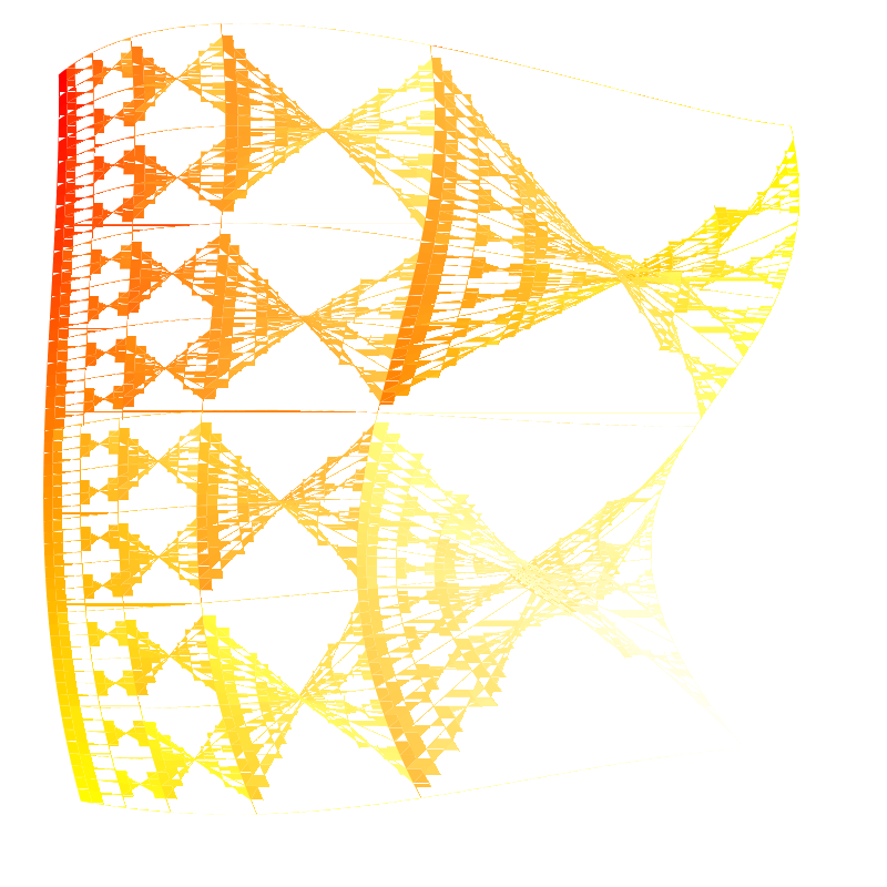
go d _northWest >> go d _northEast >> go d _southWest >> go d _southEastTo have an idea of the process, here's a GIF of various subdivision levels. At some points there is too much different colors to have a correct encoding and the dithering scramble it a bit:
What if we want to control more precisely how the color spread within a patch?
With a coon patch this is rather limited, but we have another tool to do this, the tensor patch. Here is both side by side, the coon patch on the left, the tensor patch on the right:


There is a difference of construction between the two, the Tensor patch is made of a matrix of 4x4 points with points in the middle of the matrix helping to "drag" the color one way or another:

Tensor patch debug
In the patch below, each circle represent a control point of the tensor patch, the curves defined by these points are ommited for clarity.
So a nice little tensor patch:

Which has the control mesh: (this time with curve outline drawn):

So the basic subdivision technique is to split each of the 4 cubic bezier curve in each direction:

We can then interpret the matrix in the other direction (vertically), and subdivide again the tensor patch. Here we subdivide vertically just the right patch:

We can simply switch orientation of a tensor patch by transposing its coefficients:
data TensorPatch px = TensorPatch
  { _curve0 :: !CubicBezier
  , _curve1 :: !CubicBezier
  , _curve2 :: !CubicBezier
  , _curve3 :: !CubicBezier
  , _tensorValues :: !(ParametricValues px)
  }

transposeParametricValues :: ParametricValues a -> ParametricValues a
transposeParametricValues (ParametricValues n e s w) = ParametricValues n w s e

transposePatch :: TensorPatch px -> TensorPatch px
transposePatch TensorPatch
  { _curve0 = CubicBezier c00 c01 c02 c03
  , _curve1 = CubicBezier c10 c11 c12 c13
  , _curve2 = CubicBezier c20 c21 c22 c23
  , _curve3 = CubicBezier c30 c31 c32 c33
  , _tensorValues = values
  } = TensorPatch
    { _curve0 = CubicBezier c00 c10 c20 c30
    , _curve1 = CubicBezier c01 c11 c21 c31
    , _curve2 = CubicBezier c02 c12 c22 c32
    , _curve3 = CubicBezier c03 c13 c23 c33
    , _tensorValues = transposeParametricValues values
    }
We then just have to subdivide horizontally
horizontalTensorSubdivide :: TensorPatch (V2 CoonColorWeight)
                          -> (TensorPatch (V2 CoonColorWeight), TensorPatch (V2 CoonColorWeight))
horizontalTensorSubdivide p = (TensorPatch l0 l1 l2 l3 vl, TensorPatch r0 r1 r2 r3 vr) where
  (l0, r0) = divideCubicBezier $ _curve0 p
  (l1, r1) = divideCubicBezier $ _curve1 p
  (l2, r2) = divideCubicBezier $ _curve2 p
  (l3, r3) = divideCubicBezier $ _curve3 p
  (vl, vr) = subdivideHorizontal $ _tensorValues p
And we can finally subdivide the patch in 4 subpatch:
subdivideTensorPatch :: TensorPatch (V2 CoonColorWeight)
                     -> Subdivided (TensorPatch (V2 CoonColorWeight))
subdivideTensorPatch p = subdivided where
  (west, east) = horizontalTensorSubdivide p
  (northWest, southWest) = horizontalTensorSubdivide $ transposePatch west
  (northEast, southEast) = horizontalTensorSubdivide $ transposePatch east
  subdivided = Subdivided
    { _northWest = northWest
    , _northEast = northEast
    , _southWest = southWest
    , _southEast = southEast
    }
The global rendering is similar to the one of the coon patch, so it won't be displayed here.
A tensor patch have 4 additional compared to the coon patch. It is therefore more complex, and we could pass from the coon patch to the tensor one. If \(S(u,v)\) is the point at the position u, v on the coon surface, the 4 additional points are expressed in the following way in the PDF reference 1.7, and in various articles:
\[ \begin{matrix} p11 & = & S(1/3, 1/3) \\ p21 & = & S(2/3, 1/3) \\ p12 & = & S(1/3, 2/3) \\ p22 & = & S(2/3, 2/3) \end{matrix} \]
With this, converting the following gradient mesh (expressed using the SVG2.0 Draft syntax):
<?xml version="1.0" encoding="UTF-8" standalone="no"?>
<svg xmlns="http://www.w3.org/2000/svg" xmlns:xlink="http://www.w3.org/1999/xlink"
   version="1.1" width="400" height="400">
  <defs>
    <meshgradient x="54" y="163" id="meshgradient1" gradientUnits="userSpaceOnUse">
      <meshrow>
        <meshpatch>
          <stop path="C  68, 110, 110,  68, 163,  54"  stop-color="red"    />
          <stop path="C 153,  82, 148, 111, 143, 143"  stop-color="red"    />
          <stop path="L 143, 143"                      stop-color="white " />
          <stop path="C 113, 146,  82, 153"            stop-color="white"  />
        </meshpatch>
        <meshpatch>
          <stop path="C 245,  35, 325,  83, 345, 163"                      />
          <stop path="C 281, 138, 209, 136, 143, 143"  stop-color="red"    />
          <stop path="L 143, 143"                      stop-color="white"  />
        </meshpatch>
        <meshpatch>
          <stop path="C 374, 273, 273, 374, 163, 345"                      />
          <stop path="C 138, 281, 136, 209, 143, 143"  stop-color="red"    />
          <stop path="L 143, 143"                      stop-color="white " />
        </meshpatch>
        <meshpatch>
          <stop path="C  83, 325,  35, 245,  54, 163"                      />
          <stop path="C  82, 153, 111, 148, 143, 143"  stop-color="red"    />
          <stop path="L 143, 143"                      stop-color="white " />
        </meshpatch>
       </meshrow>
     </meshgradient>
  </defs>
  <rect width="360" height="360" x="20" y="20" style="fill:url(#meshgradient1); stroke:red" />
</svg>
and render it as a bunch of tensor patches:
You can see the lines in the border of the patches, and the diamond shape of the white hallow?
Well it's total crap, even if intuitive and elegant, putting the control points at third of the bezier distance is just wrong, we can get a intuition into the problem by plotting the curve and control points of the previous rendering:
We can see the near straight line formed with the additional control points, whereas the original render is much smoother and "round". The answer is elsewhere, thanks to the one giving the pointer in the Cairo source code, indicating the ISO32000 document, an ISO standard describing the PDF format, with another set of formula to transform coon patches to tensor patches:
\[ \begin{matrix} p_{11} & = & 1/9 \times \left( -4 \times p_{00} + 6 \times (p_{01} + p_{10}) - 2 \times (p_{03} + p_{30}) + 3 \times (p_{31} + p_{13}) - 1 \times p_{33} \right) \\ p_{12} & = & 1/9 \times \left( -4 \times p_{03} + 6 \times (p_{02} + p_{13}) - 2 \times (p_{00} + p_{33}) + 3 \times (p_{32} + p_{10}) - 1 \times p_{30} \right) \\ p_{21} & = & 1/9 \times \left( -4 \times p_{30} + 6 \times (p_{31} + p_{20}) - 2 \times (p_{33} + p_{00}) + 3 \times (p_{01} + p_{23}) - 1 \times p_{03} \right) \\ p_{22} & = & 1/9 \times \left( -4 \times p_{33} + 6 \times (p_{32} + p_{23}) - 2 \times (p_{30} + p_{03}) + 3 \times (p_{02} + p_{20}) - 1 \times p_{00} \right) \end{matrix} \]
Using these new formulas, we obtain this rendering:
We can see that the control points are further from the center and we obtain a much better smoothing of the white color accross the circle:

Much better :)
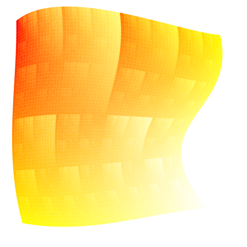
Let's return to our whole mesh gradient for a moment:
If we look at the render closely, we can see that the edges are apparent, as we use bilinear interpolation inside a patch, a neighbour patch with really different colors on the oposite vertices will create a visible discontinuity, hence the visibility of the edges.
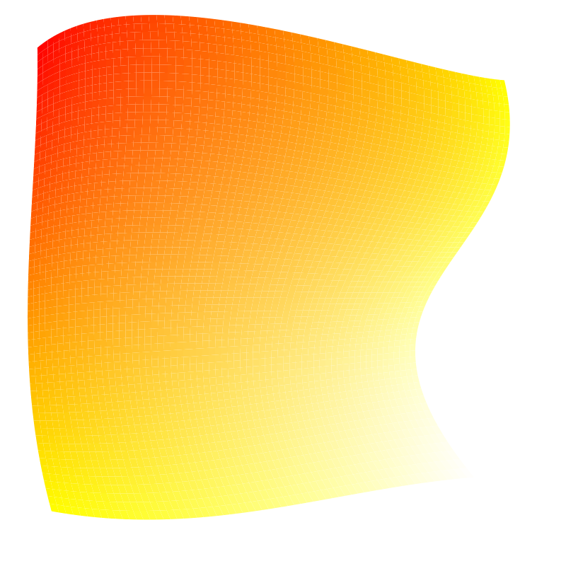
To handle this problem, the SVG2 draft document propose to choose between two interpolation scheme for rendering: bilinear and bicubic (bilinear being the default one). Using the bicubic method, we obtain a much smoother rendering:

We can still see the mesh edges on certain cases, but it's globally smoother. We can use the parametricity of our types to switch from a normal mesh patch to a one that will interpolate with cubic interpolation. We can first store the slope information at every vertice of the mesh:
-- | Store the derivative necessary for cubic interpolation in
-- the gradient mesh. We use tiny vectors because we need coefficients
-- for every color component in the image.
data Derivative px = Derivative
  { _derivValues  :: !(V4 Float)
  , _xDerivative  :: !(V4 Float)
  , _yDerivative  :: !(V4 Float)
  , _xyDerivative :: !(V4 Float)
  }

-- | Prepare a gradient mesh to use cubic color interpolation, see
-- renderCubicMesh documentation to see the global use of this function.
calculateMeshColorDerivative :: MeshPatch PixelRGBA8 -> MeshPatch (Derivative pPixelRGBA8)
calculateMeshColorDerivative mesh = mesh { _meshColors = colorDerivatives } where
  colorDerivatives =
     V.fromListN (w * h) [interiorDerivative x y | y <- [0 .. h - 1], x <- [0 .. w - 1]]

  w = _meshPatchWidth mesh + 1
  h = _meshPatchHeight mesh + 1
  clampX = max 0 . min (w - 1)
  clampY = max 0 . min (h - 1)
  toFloatPixel (PixelRGBA8 r g b a) =
    V4 (fromIntegral r) (fromIntegral g) (fromIntegral b) (fromIntegral a)

  rawColorAt x y =_meshColors mesh V.! (y * w + x)
  atColor x y = toFloatPixel $ rawColorAt (clampX x) (clampY y)
  pointAt x y = verticeAt mesh (clampX x) (clampY y)
  derivAt x y = colorDerivatives  V.! (y * w + x)

  interiorDerivative x y = Derivative thisColor dx dy dxy
    where
      dx = slopeBasic cxPrev cxNext xPrev xNext
      dy = slopeBasic cyPrev cyNext yPrev yNext

      dxy | nearZero xyDist = zero
          | otherwise = (cxyNext ^-^ cyxPrev ^-^ cyxNext ^+^ cxyPrev) ^/ (xyDist)
      xyDist = (xNext `distance` xPrev) * (yNext `distance` yPrev)

      cxyPrev = atColor (x - 1) (y - 1)
      xyPrev = pointAt (x - 1) (y - 1)

      cxyNext = atColor (x + 1) (y + 1)
      xyNext = pointAt (x + 1) (y + 1)

      cyxPrev = atColor (x - 1) (y + 1)
      yxPrev = pointAt (x - 1) (y + 1)

      cyxNext = atColor (x + 1) (y - 1)
      yxNext = pointAt (x + 1) (y - 1)

      cxPrev = atColor (x - 1) y
      thisColor = atColor x y
      cxNext = atColor (x + 1) y

      cyPrev = atColor x (y - 1)
      cyNext = atColor x (y + 1)

      xPrev = pointAt (x - 1) y
      this  = pointAt x y
      xNext = pointAt (x + 1) y

      yPrev = pointAt x (y - 1)
      yNext = pointAt x (y + 1)
And when extracting a single patch, use the calculation used in the Wikipedia article to compute the final coefficients of our interpolation:
-- | Store information for cubic interpolation in a patch.
newtype CubicCoefficient px = CubicCoefficient
    { getCubicCoefficients :: ParametricValues (V4 (V4 Float))
    }

rawMatrix :: V.Vector (V.Vector Float)
rawMatrix = V.fromListN 16 $ V.fromListN 16 <$>
  [ [ 1, 0, 0, 0,  0, 0, 0, 0,  0, 0, 0, 0,  0, 0, 0, 0 ]
  , [ 0, 0, 0, 0,  1, 0, 0, 0,  0, 0, 0, 0,  0, 0, 0, 0 ]
  , [-3, 3, 0, 0, -2,-1, 0, 0,  0, 0, 0, 0,  0, 0, 0, 0 ]
  , [ 2,-2, 0, 0,  1, 1, 0, 0,  0, 0, 0, 0,  0, 0, 0, 0 ]
  , [ 0, 0, 0, 0,  0, 0, 0, 0,  1, 0, 0, 0,  0, 0, 0, 0 ]
  , [ 0, 0, 0, 0,  0, 0, 0, 0,  0, 0, 0, 0,  1, 0, 0, 0 ]
  , [ 0, 0, 0, 0,  0, 0, 0, 0, -3, 3, 0, 0, -2,-1, 0, 0 ]
  , [ 0, 0, 0, 0,  0, 0, 0, 0,  2,-2, 0, 0,  1, 1, 0, 0 ]
  , [-3, 0, 3, 0,  0, 0, 0, 0, -2, 0,-1, 0,  0, 0, 0, 0 ]
  , [ 0, 0, 0, 0, -3, 0, 3, 0,  0, 0, 0, 0, -2, 0,-1, 0 ]
  , [ 9,-9,-9, 9,  6, 3,-6,-3,  6,-6, 3,-3,  4, 2, 2, 1 ]
  , [-6, 6, 6,-6, -3,-3, 3, 3, -4, 4,-2, 2, -2,-2,-1,-1 ]
  , [ 2, 0,-2, 0,  0, 0, 0, 0,  1, 0, 1, 0,  0, 0, 0, 0 ]
  , [ 0, 0, 0, 0,  2, 0,-2, 0,  0, 0, 0, 0,  1, 0, 1, 0 ]
  , [-6, 6, 6,-6, -4,-2, 4, 2, -3, 3,-3, 3, -2,-1,-2,-1 ]
  , [ 4,-4,-4, 4,  2, 2,-2,-2,  2,-2, 2,-2,  1, 1, 1, 1 ]
  ]

cubicPreparator :: ParametricValues (Derivative PixelRGBA8)
                -> CubicCoefficient PixelRGBA8
cubicPreparator ParametricValues { .. } =
    CubicCoefficient $ ParametricValues (sliceAt 0) (sliceAt 4) (sliceAt 8) (sliceAt 12) where
  Derivative c00 fx00 fy00 fxy00 = _northValue
  Derivative c10 fx10 fy10 fxy10 = _eastValue
  Derivative c01 fx01 fy01 fxy01 = _westValue
  Derivative c11 fx11 fy11 fxy11 = _southValue

  resultVector = mulVec $ V.fromListN 16
    [  c00,   c10,   c01,   c11
    , fx00,  fx10,  fx01,  fx11
    , fy00,  fy10,  fy01,  fy11
    ,fxy00, fxy10, fxy01, fxy11
    ]

  mulVec vec = VG.foldl' (^+^) zero . VG.zipWith (^*) vec <$> rawMatrix

  sliceAt i = V4
    (resultVector V.! i)
    (resultVector V.! (i + 1))
    (resultVector V.! (i + 2))
    (resultVector V.! (i + 3))
Storing the cubic coefficients in a V4 is a bit a hacky way to do it, but it let us store a 16 element vector easily. Finally to let us render the patch with the correct interpolation, we can roll a new instance of BiSampleable, just making a big dot product between the coefficients and our current position.
-- | Bicubic interpolator
instance BiSampleable (CubicCoefficient PixelRGBA8) PixelRGBA8 where
interpolate = bicubicInterpolation
bicubicInterpolation :: CubicCoefficient PixelRGBA8 -> Float -> Float -> PixelRGBA8
bicubicInterpolation params x y =
fromFloatPixel . fmap clamp $ af ^+^ bf ^+^ cf ^+^ df
where
ParametricValues a b c d = getCubicCoefficients params
clamp = max 0 . min 255
-- we are really doing the dot product of two vector by hand, but
-- each element is not a scalar but a 4 element vector representing
-- the color
xv, vy, vyy, vyyy :: V4 Float
xv = V4 1 x (x*x) (x*x*x)
vy = xv ^* y
vyy = vy ^* y
vyyy = vyy ^* y
v1 ^^*^ v2 = (^*) <$> v1 <*> v2
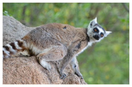
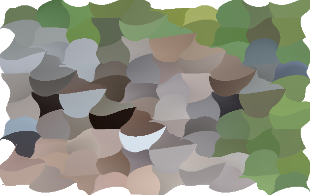
V4 af bf cf df = (a ^^*^ xv) ^+^ (b ^^*^ vy) ^+^ (c ^^*^ vyy) ^+^ (d ^^*^ vyyy)Ok, enough with interpolations, let's try something else. We're going to start with a picture:
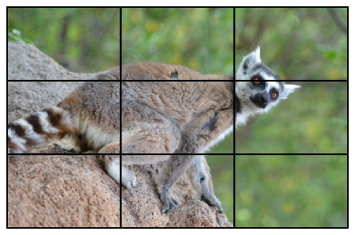
Put a conceptual mesh grid on top of this image
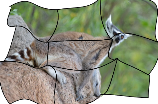
Shake the vertices of the mesh
And voilà, a wonderful distorted image:
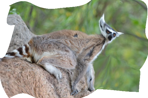
Any resemblance to previous techniques is purely indented. Sadly this part is not in the SVG2 draft spec.
Each patch interpolate within [0, 1]², so instead of interpolating between the four corner colors, we can just fetch pixels from an image. To store the information of a patch we need a new data type:
-- | Type storing the information to be able to interpolate
-- part of an image in a patch.
data ImageMesh px = ImageMesh
    { _meshImage :: !(Image px)
    , _meshTransform :: !Transformation
    }
The transformation is there to change space from the UV parametric space to the image space, and just fetch the pixel at the good position. I'll spare the implementation as there is not that much to do here, but it all boil down to just a new instance of BiSampleable
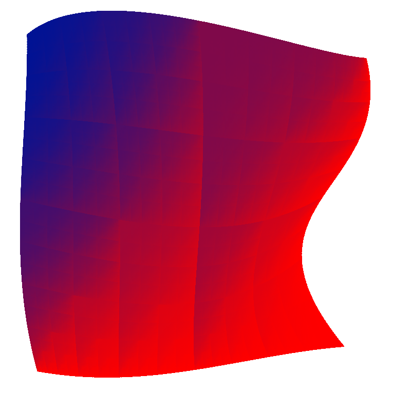
If you forget to transform, you're in for a weird image with many patches:
So, we have a simple implementation relying only on subdivision, and heavy subdivision is not that cheap and can result on some massive overdraw if not tuned properly (like in the code given in the sections above). And the result are not that great when interpolating an image.
So we can't really rely only on this algorithm for rendering. The real algorithm in use in Rasterific right now is the Fast Forward Differencing (explained in details on scratchapixel).
With this algorithm, you go from the parametric version of the cubic bezier curve:
\[ P(t) = P _ 0 (1 - t) ^ 3 + 3 P _ 1 t (1 - t) ^ 2 + 3 P _ 2 t^2 (1 - t) + P_3 t ^ 3 \]
to three addition between each pixel (more or less).
The core of the algorithm is to be able to go to step \(n\) to step \(n+1\) with small steps, doing that with only one level will only give us a straight line, as we're playing with a cubic equation, we will have to apply multiple time the forward differentiation operator.
The forward difference operator is defined as: \[ ffd(f, t) = f(t + h) - f(t) \]
Where \(h\) is the step size open to choice. We are interested to setup the coefficients for the first point of the curve (ie. for \(t = 0\)), and initially, we initially want a step of 1, thus:
So using the bezier equation:
\[ P(t) = P _ 0 (1 - t) ^ 3 + 3 P _ 1 t (1 - t) ^ 2 + 3 P _ 2 t^2 (1 - t) + P_3 t ^ 3 \]
With a bit of rewriting (and the help of sympy to perform symbolic computations), we obtain:
\[ ffd_1(t) = ffd(P, t) = - h^3 p_0 + 3 h^3 p_1 - 3 h^3 p_2 + \\ h^3 p_3 + 3 h^2 p_0 - 6 h^2 p_1 + 3 h^2 p_2 - 3 h p_0 + \\ 3 h p_1 + t^2 (- 3 h p_0 + 9 h p_1 - 9 h p_2 + 3 h p_3) + \\ t (- 3 h^2 p_0 + 9 h^2 p_1 - 9 h^2 p_2 + 3 h^2 p_3 + \\ 6 h p_0 - 12 h p_1 + 6 h p_2) \]
which simplify to
\[ ffd_1(0) = - p_0 + p_3 \]
in our case
In a similar way, we calculate second and third order differentiation:
\[ \begin{matrix} ffd_2(t) & = & ffd(ffd_1, t) \\ ffd_2(0) & = & 6 p_1 - 12 p_2 + 6 p_3 \end{matrix} \]
And
\[ \begin{matrix} ffd_3(t) & = & ffd(ffd_2, t) \\ ffd_3(0) & = & - 6 p_0 + 18 p_1 - 18 p_2 + 6 p_3 \end{matrix} \]
We can try to calculate the fourth order, but it won't yield anything:
\[ ffd_4(t) = ffd(ffd_3, t) = 0 \]
So we can stop.
So using this information, we set up our initial coefficients
\[ \begin{matrix} X & = & x_0 \\ A & = & ffd_1(0) \\ B & = & ffd_2(0) \\ C & = & ffd_3(0) \end{matrix} \]
And we can make an step evaluation step with a simple summation:
\[ \begin{matrix} X' & = & X + A \\ A' & = & A + B \\ B' & = & B + C \\ C' & = & C \end{matrix} \]
Which is a far cheaper computation ### Cubic bezier rasterization using Forward difference
With these tools at hand, we can now write down data structure and conversion functions.
data ForwardDifferenceCoefficient = ForwardDifferenceCoefficient
    { _fdA :: {-# UNPACK #-} !Float
    , _fdB :: {-# UNPACK #-} !Float
    , _fdC :: {-# UNPACK #-} !Float
    }

-- | Given a cubic curve, return the initial step size and
-- the coefficient for the forward difference.
-- Initial step is assumed to be "1"
bezierToForwardDifferenceCoeff
    :: CubicBezier
    -> V2 ForwardDifferenceCoefficient
bezierToForwardDifferenceCoeff (CubicBezier x y z w) = V2 xCoeffs yCoeffs
  where
    xCoeffs = ForwardDifferenceCoefficient { _fdA = ax, _fdB = bx, _fdC = cx }
    yCoeffs = ForwardDifferenceCoefficient { _fdA = ay, _fdB = by, _fdC = cy }

    V2 ax ay = w ^-^ x -- ffd_1
    V2 bx by = (w ^-^ z ^* 2 ^+^ y) ^* 6 -- ffd_2
    V2 cx cy = (w ^-^ z ^* 3 ^+^ y ^* 3 ^-^ x) ^* 6 -- ffd_3

halveFDCoefficients :: ForwardDifferenceCoefficient -> ForwardDifferenceCoefficient
halveFDCoefficients (ForwardDifferenceCoefficient a b c) =
    ForwardDifferenceCoefficient { _fdA = a', _fdB = b', _fdC = c' }
  where
    c' = c * 0.125          -- c * 0.5 ^ 3
    b' = b * 0.25 - c'      -- b * 0.5 ^ 2 - c * 0.5 ^ 3
    a' = (a - b') * 0.5
We used \(h = 1\) to simplify the calculations, which is far too big for our purpose, so we can halves the coefficients after to get almost a pixel per step (see [1])
updateForwardDifferencing :: ForwardDifferenceCoefficient -> ForwardDifferenceCoefficient
updateForwardDifferencing (ForwardDifferenceCoefficient a b c) =
  ForwardDifferenceCoefficient (a + b) (b + c) c

updatePointsAndCoeff :: (Applicative f', Applicative f, Additive f)
                     => f' (f Float) -> f' (f ForwardDifferenceCoefficient)
                     -> (f' (f Float), f' (f ForwardDifferenceCoefficient))
updatePointsAndCoeff pts coeffs =
    (advancePoint <$> pts <*> coeffs, fmap updateForwardDifferencing <$> coeffs)
  where
    fstOf (ForwardDifferenceCoefficient a _ _) = a
    advancePoint v c = v ^+^ (fstOf <$> c)
rasterizerCubicBezier :: (PrimMonad m, ModulablePixel px, BiSampleable src px)
                      => src -> CubicBezier -> UV -> UV -> DrawContext m px ()
rasterizerCubicBezier source bez uvStart uvEnd = do
  canvas <- get
  let baseFfd = bezierToForwardDifferenceCoeff bez
      shiftCount = estimateFDStepCount bez
      maxStepCount :: Int
      maxStepCount = 1 `unsafeShiftL` shiftCount
      coeffStart = fixIter shiftCount halveFDCoefficients <$> baseFfd
      V2 du dv = (uvEnd ^-^ uvStart) ^/ fromIntegral maxStepCount

      go !currentStep _ _ _ _
        | currentStep >= maxStepCount = return ()
      go !currentStep !coeffs !p@(V1 (V2 x y)) !u !v = do
        let !(pNext, coeffNext) = updatePointsAndCoeff p coeffs
            !color = interpolate source (V2 u v)
        plotPixel canvas color (floor x) (floor y)
        go (currentStep + 1) coeffNext pNext (u + du) (v + dv)

  lift $ go 0 (V1 coeffStart) (V1 $ _cBezierX0 bez) du dv
To render our tensor patch, we interpolate accross the 4 cubic bezier of the patch in one direction, and rasterize a curve made of the 4 current point at each positions, yielding the final render.
So here is the end of our journey into the gradient mesh rendering for SVG2, these features will be released with the Rasterific 0.7 and the associated packages (svg-tree & rasterific-svg). So let's hope browser implement quickly the support for this new feature to allow more usage of this interesting gradient object.
Glitches are a nice, here's a collection of the nicest ones:
The grid appearing in the picture above is what happen when we don't disable anti aliasing.
[1] Chengfu Yao, Jon Rokne An efficient algorithm for subdividing linear Coons surfaces Article in Computer Aided Geometric Design 8(4):291-303 · October 1991
[2] Paul S. Heckbert, Bilinear Coons Patch Image Warping Graphics Gems IV, pages{438--446}, 1994
[3] Lien, Shantz and Pratt "Adaptive Forward Differencing for Rendering Curves and Surfaces"
[4] [Cairo](https://www.cairographics.org/)